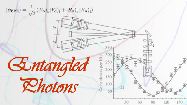
In 2002, Dietrich Dehlinger and M. W. Mitchell posted a paper called “Entangled photons, nonlocality and Bell inequalities in the undergraduate laboratory”. A closer look at this paper allows us to test and refine any Quantum Entanglement model.

Alice and Bob – Entangled Photons

The experiment described and performed by Dehlinger and Mitchell centers around the detection of photon pairs at two different locations. The polarization of a photon stream is first fixed in a specific direction from vertical with a linear polarizer, then the phase of one component is fixed with a birefringent quartz plate. The photon stream is then directed at beta barium borate (BBO) crystals that cause a small fraction of the laser photons to spontaneously decay into photon pairs with the same total energy as the original photon (a process called spontaneous parametric downconversion).

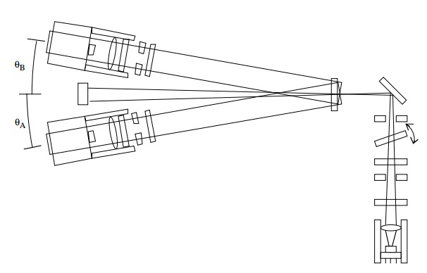
Two single-photon counting modules (SPCMs), are used to detect the photons. One detector is traditionally named Bob and the other Alice. Because the photons of a downconverted pair are produced at the same time they cause coincident, i.e., nearly simultaneous, firings of the SPCMs. Simultaneous firings are considered coincidences if they occur within 25 nanoseconds of each other. The experiment is done by recording the number of coincidences that occur for various settings for the measurement angle of Bob and Alices detectors. The number of coincidences at different observer angles is what must be modelled correctly as a “local realistic hidden variable theory” (HVT).

Modelling Entangled Photons – Close but not Quite

Dehlinger and Mitchell propose a model where each photon has a polarization angle λ. When a photon meets a polarizer set to an angle γ , it will always register as Vγ if λ is closer to γ than to γ + π/2, i.e.,

• if |γ − λ| ≤ π/4 then vertical
• if |γ − λ| > 3π/4 then vertical
• horizontal otherwise.

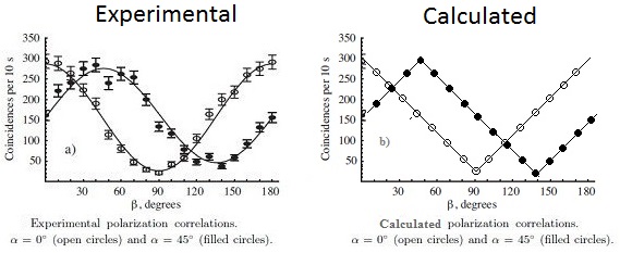
Dehlinger and Mitchell go on to generate their experimental results and generate the graphic below on the left. The open circles representing Alice at 0° and Bob at 0 to 180°. The closed circles represent Alice settings at 45° and Bob at 0 to 180°.

Represented by icons, the model is plotted against the same angles and produces results shown as calculated on the right. Clearly the calculated results differ from the experimental results. The angle 22.5° shows the most difference between the model and experiment. Dehlinger and Mitchell choose this angle to analyse in detail and show that their experimental results match with quantum physics. In their words “Our HVT is very simple, and yet it agrees pretty well with quantum mechanics. We might hope that some slight modification would bring it into perfect agreement.”.

Refining the Model – adding Probability

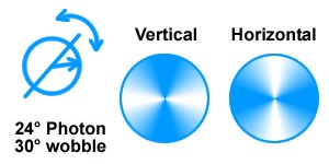
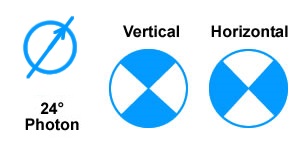
To make the model a little more accurate, Animated Physics models the photons as not only having a specific “average” direction, but also as having a “wobble” or “instantaneous” direction. Represented as icons, photons present a more “fuzzy” picture of their polarization. The sample 24° photon, with a 30° wobble, will most of the time be picked up as a vertical, but sometimes when the combined angle is over 45°, it will be picked up as a horizontal. To determine polarity, we use these equations.

• Chance of vertical measurement = (cos((γ − λ)*2)+1)/2
• Chance of horizontal measurement = (cos((γ − λ + π/2)*2)+1)/2

Now consider some angles. A horizontal photon has a 100% chance of getting through a horizontal polarizer. A vertical photon has 0% chance of getting through a horizontal polarizer.

A photon with a polarization angle of 45° has a 50% chance of getting through a horizontal polarizer and a 50% chance of getting through a vertical polarizer. Finally, a photon with polarization angle of 22.5° has a 85% chance of getting through a horizontal polarizer and a 15% chance of getting through a vertical polarizer.

Visualizing the Entanglement Model

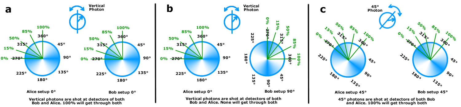
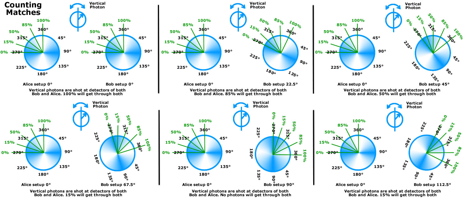
Let’s start the experiment. To calibrate the equipment, we test that Alice and Bob get maximum matches with both set at 0° (a), they get minimum matches with Alice at 0° and Bob at 90° since the vertical photons have no chance of getting though Bob’s filter (b), with the photon stream set to 45°, Bob and Alice match all photons when both set to 45° (c). The green numbers represent the probability of a photon getting through at that angle.

With the equipment calibrated, we fix the polarizer that Alice is using at 0°, and rotate Bob’s polarizer through a variety of angles and collect our data.

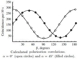
These results demonstrates that this model matches the results of experiment. In fact, the model follows the same cos(γ − λ)² rule that is used by quantum mechanics.

To have fun playing around with photon polarization settings as well as filter angles, click on “Shoot the Photon”.