In his Autobiographical Notes in 1949, Einstein wrote of the special theory

It is striking that the theory introduces two kinds of physical things, i.e., (1) measuring rods and clocks, and (2) all other things, e.g., the electromagnetic field, the material point, etc.

In the last blog entry, we set the measuring rods to picometers (10‾¹²) and our clocks to attoseconds (10‾¹⁸) . We got a nice view of electrons buzzing around under the coulomb force with energies in the range of 13.6 eVolts and speeds around 2.2 picometers per attosecond (have a look and play Shoot the Electron).

What we could not see is any significant motion of the protons. The protons and other nucleons, being thousands of times heavier then the electron, sit there while the electrons buzz around. To see any motion of the proton, we must put the animation into super fast-forward mode.  Specifically, we leave our measuring rods at picometers (10‾¹²) but move our clocks to femtoseconds (10‾¹⁵).

Hydrogen Atomic Orbitals

The view of the atom at the femtosecond time scale is dramatically different from the view of the atom at the attosecond time scale. At the attosecond time scale (10‾¹⁸), we were able to model movements of low energy electrons buzzing around.  At the femtosecond time scale (10‾¹⁵), it makes no sense to track the electrons movement, but rather there is a cloud of probability of where the electron could be. In more general terms, we see a specific area that electrons become confined to and their attractive effect on the proton is really coming from the whole area. At this speed, the view of the proton remains much the same, but now it has the ability to move around. Protons and other nucleons are capable of breaking and/or forming new bonds with other protons and nucleons through ever changing clouds of atomic orbitals.

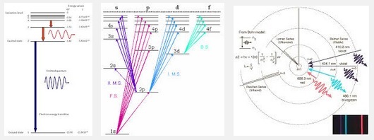A quick google search of “hydrogen energy levels”, produces a variety of different styles to represent the relationship between electron bonding and the emission or absorption of photons of specific energy. To properly model the atom, we must track what energy levels are filled over time as electrons fall into atoms, emitting photons and becoming bonded to the atom at a specific energy level.

Atomic orbitals are calculated from mathematical wave functions that predict the probability of finding an electron or a pair of electrons in a specific region around the atom’s nucleus. Quantum mechanics tells us that electrons in an atom possess four quantum numbers that determine what energy level the electron is at. They are: Orbital (harmonic overtones), n=1,2,3…; Azimuthal (location on sphere), l=0,1,2…n−1; Magnetic (electron coupling), ml=−l,−l+1…0…l−1,l; and finally Spin (up and down), ms=−1/2,1/2. The first two quantum numbers determine location, the third number specifies the magnetic coupling between electrons, and the last quantum number, spin, is a property of the electron itself.

If we have some electrons that need to be filled into the energy levels, we start with shell n=0, with l=0 and ml=0, and with ms=-1/2 or +1/2 (2 S-electrons). For shell n=1, starting with l=0, we have ml=0 and ms=-1/2 or +1/2 (2 S-electrons). Also for n=1, with l=1 allows ml=-1, 0 and 1, with each ms=-1/2 or +1/2 (6 P-electrons).

The image on the right provides a summary of what to track. The Azimuthal (l) represents a location on the surface of a vibrating sphere. The Orbital (n) represents the overtones of the fundamental vibrations. All of the possible energy levels are indicated and we color a dot red to indicate an electron is there; and, add a line to the center to indicate the bond. In this image, it is important to remember the dots are representing orbitals, and the image has been squished into a 2D representation.

Click here to view a 3D representation of this same style for a neon atom. A neon atom has a complete set of electrons in the first two energy levels, filling all 10 spots for S1, S2 and P2 electrons. It’s fun to rotate the 3D image and line up a pair of P2 electrons. Notice the other P2 electrons form a natural xyz grid in 3 dimensions. The S-electrons represent spherical orbitals while the P-electrons represent nodes on opposite sides of the nucleon. If you think of the P-electrons as 3 distinct pairs, you get ml=-1, 0 and 1. These observations are important to move in towards modeling more complex particles containing bonded components of other more simple particles.

Coming next: Putting a model in action – an animation of the energy levels, photon emissions and absorption in the Helium/Neon laser.